About

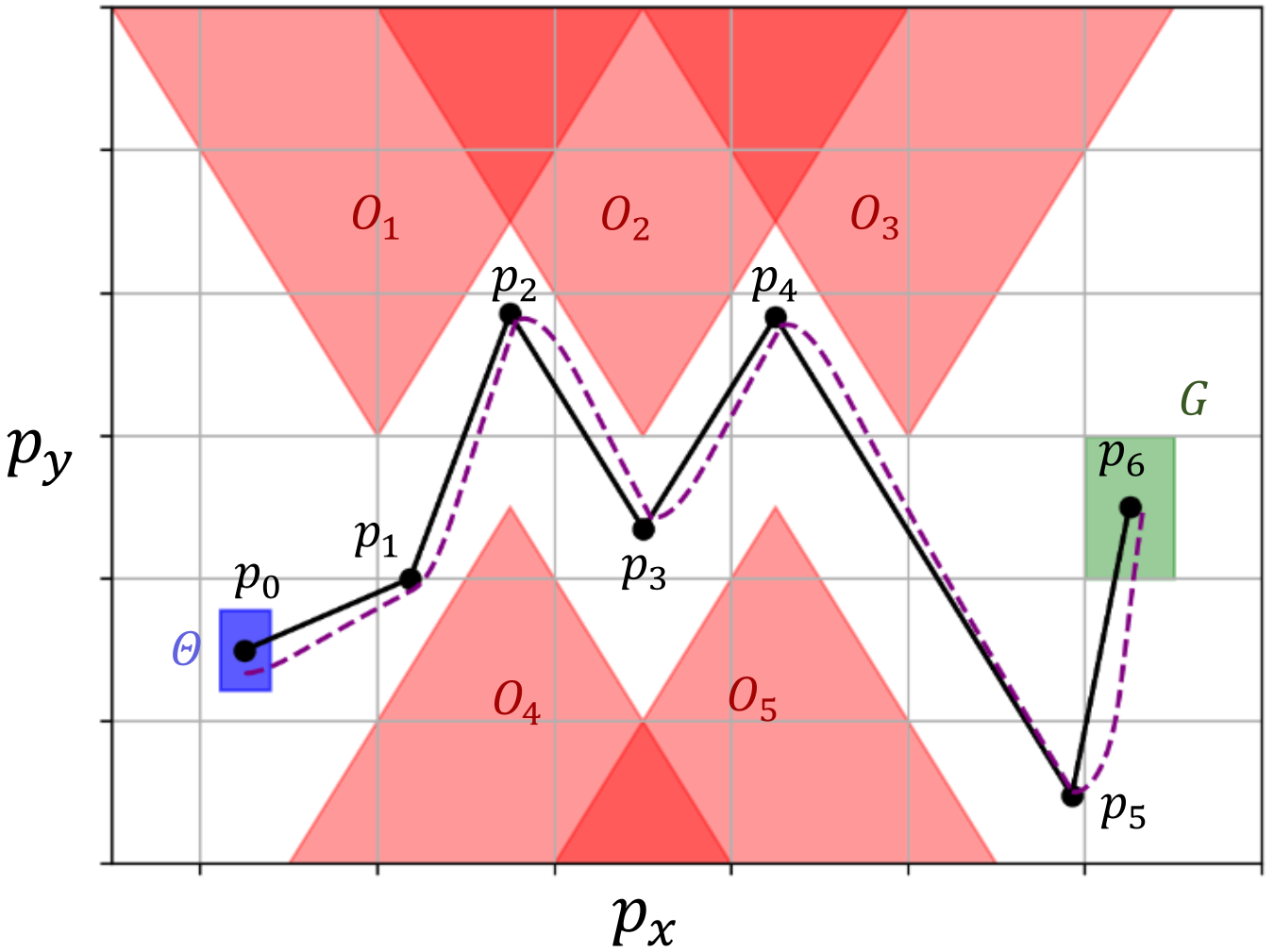
FACTEST is a controller synthesis tool for nonlinear systems. Specifically, it solves reach-avoid scenarios for vehicular models. An example can be seen in the image below. The obstacles are shown in red, the initial set is shown in blue, and the goal set is shown in green. The reference trajectory returned by FACTEST is represented by the solid black line. The actual trajectory that the system follows is shown by the dotted purple line.

The inputs to FACTEST are as follows: an environment, a model, and a maximum number of segments. The output is a reference controller. This makes it very simple to create your own scenarios to be solved by FACTEST. The documentation for using FACTEST can be found on the GitHub page.

To get a better understanding of how FACTEST works, a brief tutorial will be provided on this page. However, it is highly recommended that you read the papers associated with FACTEST. These papers can be found here.

Example

Step 1. Define Environment

Let us consider the reach avoid scenario presented in the figure above. The obstacles, initial set, and goal set are all represented as polytopes. The environment is then defined as the following:

Obstacles:

\( \begin{bmatrix} -1 & 1 \\ 1 & 1 \\ 0 & 1 \end{bmatrix} x \leq \begin{bmatrix} 0.5 \\ 2 \\ 0 \end{bmatrix} \), \( \begin{bmatrix} -1 & 1 \\ 1 & 1 \\ 0 & 1 \end{bmatrix} x \leq \begin{bmatrix} -1 \\ 3.5 \\ 0 \end{bmatrix} \), \( \begin{bmatrix} -1 & -1 \\ 1 & -1 \\ 0 & 1 \end{bmatrix} x \leq \begin{bmatrix} -3 \\ 0 \\ 3 \end{bmatrix} \), \( \begin{bmatrix} -1 & -1 \\ 1 & -1 \\ 0 & 1 \end{bmatrix} x \leq \begin{bmatrix} -1.5 \\ -1.5 \\ 3 \end{bmatrix} \), \( \begin{bmatrix} -1 & -1 \\ 1 & -1 \\ 0 & 1 \end{bmatrix} x \leq \begin{bmatrix} -4.5 \\ 1.5 \\ 3 \end{bmatrix} \)

Borders(included in the obstacle list):

\( \begin{bmatrix} -1 & 0 \\ 1 & 0 \\ 0 & -1 \\ 0 & 1 \end{bmatrix} x \leq \begin{bmatrix} 1.5 \\ 5 \\ 0.1 \\ 0 \end{bmatrix} \), \( \begin{bmatrix} -1 & 0 \\ 1 & 0 \\ 0 & -1 \\ 0 & 1 \end{bmatrix} x \leq \begin{bmatrix} 1.5 \\ 5 \\ -3 \\ 3.1 \end{bmatrix} \), \( \begin{bmatrix} -1 & 0 \\ 1 & 0 \\ 0 & -1 \\ 0 & 1 \end{bmatrix} x \leq \begin{bmatrix} 1.6 \\ -1.5 \\ 0 \\ 3 \end{bmatrix} \), \( \begin{bmatrix} -1 & 0 \\ 1 & 0 \\ 0 & -1 \\ 0 & 1 \end{bmatrix} x \leq \begin{bmatrix} -5 \\ 5.1 \\ 0 \\ 3 \end{bmatrix} \)

Initial Set \(\Theta\):

\( \begin{bmatrix} -1 & 0 \\ 1 & 0 \\ 0 & -1 \\ 0 & 1 \end{bmatrix} x \leq \begin{bmatrix} 0.9 \\ -0.6 \\ 0.6 \\ 0.9 \end{bmatrix} \)

Goal Set:

\( \begin{bmatrix} -1 & 0 \\ 1 & 0 \\ 0 & -1 \\ 0 & 1 \end{bmatrix} x \leq \begin{bmatrix} -4 \\ 4.5 \\ -1 \\ 1.5 \end{bmatrix} \)

Step 2. Define model

The model used to navigate the reach-avoid scenario is the rearwheel kinematic car model. A tracking controller is needed to track the reference trajectory returned by FACTEST. A Lyapunov-based feedback controller is chosen. The dynamics of the car model and the control law are shown below:

Dynamics:

\[ \dot{p} = \begin{bmatrix} \dot{x} \\ \dot{y} \\ \dot{\theta} \end{bmatrix} x = \begin{bmatrix} v \sin(\theta) \\ v \cos(\theta) \\ \omega \end{bmatrix} \]

Tracking Controller Law:

\[ v = v_{ref} \cos(e_{\theta}) + k_1 e_x \] \[ \omega = \omega_{ref} + v_{ref}(k_2 e_y + k_3 \sin(e_{\theta})) \]

Step 3. Compute Error Bounds

The next step is to compute the error bounds of the actual trajectory from the reference trajectory. Since a Lyapunov-based controller was chosen, the error can be bounded using Lyapunov sublevel sets. This is discussed more in depth in this paper. The error bounds can also be computed using reachability analysis, as proposed in this paper. For this example, the bounds will be computed using the Lyapunov-based analysis. The size of the error bound is shown below:

Error Bounds:

\[ \ell(n) = \sqrt{\ell_0^2 + \frac{4n}{k_2}} \quad n=0,1,\cdots,N-1 \] where \(\ell_0\) is the size of the initial set, and \(N\) is the maximum number of line segments.

Step 4. Compute Reference Controller

Once the error bounds are computed, the reference controller can be found. This is done in 2 steps: finding a reference path, then converting that path to a reference trajectory. Finding the reference path can be done by either solving a SAT problem or a MILP problem. The path \( \xi_{ref}(t) \) is returned as a piecewise linear path. Once the path is found, it is converted to a reference trajectory and the reference controller \( u_{ref}(t) \) is computed. The reference controller is returned as \( [\Theta, t, \xi_{ref}, u_{ref}] \) . The returned reference controller is guaranteed safe for any trajectory starting in the initial set. If the reference controller is fed to the system defined in step 2, then an example trajectory is shown below:

Solution:

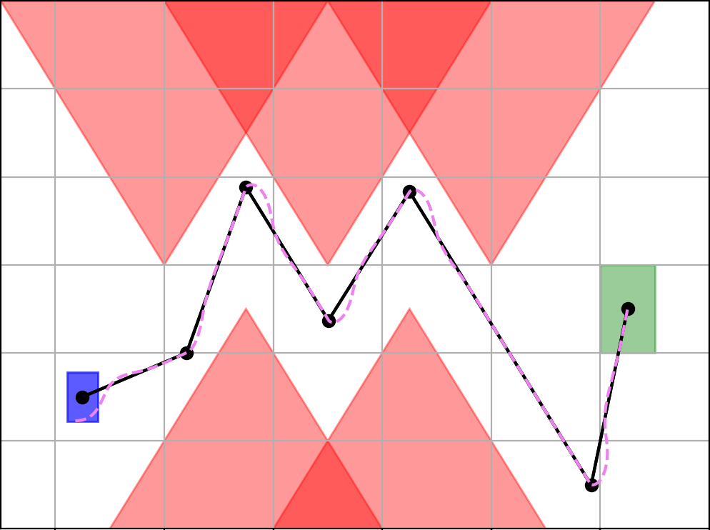
Example solution to the reach-avoid scenario